The Sunday blog: Boost your HMI with advanced mathematics! – Part 3: Drawing curves

The Sunday blog: Boost your HMI with advanced mathematics!

Part 3: Drawing curves

After much theory about fixed point math in the previous episode, let’s just recall a fey things, before we move on to drawing polynomial curves in practice:

• Multiplication will double the number of significant bits, therefore, we can use a maximum of 16bits as a factor on a 32bit system.
• The highest precision will be obtained with the q15 format which uses 1 sign bit and 15 fraction bits. It’s ideal for trigonometric computation at highest precision, but since there are no integer bits, we are restricted to the range from -1 to +1 if we don’t want to run into digit loss through multiplication overflow.
• In other mathematical applications, we’ll have to make a choice between precision and range. The higher the needed range, the lower the precision. We’ll see below which considerations come into play.
• The corresponding HMI file with all code and graphic resources can be downloaded in the Nextion forums.

Drawing or plotting ?

Plotting is obviously the easiest way. Take an x value, calculate the y value, set a point in (x,y) and you are done. But plotting a curve this way might give ugly results, i.e. if for consecutive x values, the y values vary strongly, there will be a huge blank between the consecutive dots and it will be difficult to see the curve. That’s why most times, drawing which means using a line from the previous to the actual point. It makes your code slightly more complex since you need 2 additional variables to keep the previous x and y values and you have to take care to draw your line only from the second iteration on. But the gain in graphic quality is worth it.

The “canvas” to draw on

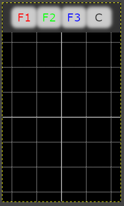
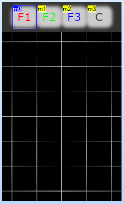As seen in an earlier blog, putting all static content into the page background simplifies the HMI design greatly. Thus, we’ll open our graphics program, i.e. Gimp, place 4 symbolic buttons, 3 for our demo functions and one to clear the screen, and add a 240*340px virtual screen with an oscilloscope-like grid. After exporting it as a bmp in RGB-565 color encoding, it can directly be imported as a picture resource in the Nextion editor and is used as the background of page0. We’ll add 4 hotspots above the 4 symbolic buttons to make them real ones.

The mathematical origin, the center point of our drawing canvas has the absolute pixel coordinates x0=120 and y0=230. We further keep the numbers small to get a maximum of precision, thus we define that 1 be represented by 100 pixel which is two of our grid lines. The x range goes thus from -1.2 to 1.2 and the y range from -1.7 to 1.7. With these definitions (all in the program.s file), we can proceed to the precision considerations: Selecting the q12 format allows us to operate in the -8 to 8 range with 12 fractional bits which leaves some headroom while the precision remains high enough with 1/4096 or 0.024%. These details are defined in program.s, too, so that our function drawing routines remain small, efficient, and flexible though:

// pseudo-constant for fixed point math (using q12 in this project)
int q_shift=12
// display scaling (100px/unit) and origin
int d_scale=100, x0=120,y0=230
// variables for line drawing:
int x_last=0,x_cur=0,y_last=0,y_cur=0,run=0
// declare helpers
int x,y
int x_step,x_start,x_end
x_step=1<<q_shift+50/d_scale // rounded 100 steps per unit
x_start=-6<<q_shift/5 // -1.2 in q12
x_end=6<<q_shift/5 // 1.2 in q12

The curves to draw

To fit nicely into our drawing screen, we define the following functions:
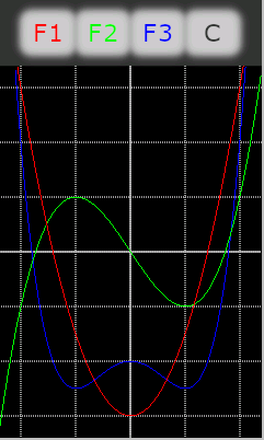
(You’ll find that everything is drawn upside down because on the HMI, positive y go downwards while in mathematics, they go upwards. That’s why the sign of all coefficients is reversed here)

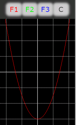
F1: y = -3.0x^2 + 1.5
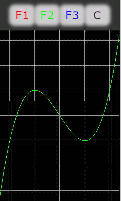
F2: y = -2.0x^3 + 1.5x
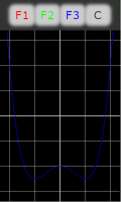
F3: y = -4.0x^4 + 2.0x^2 + 1.0

The corresponding polynomial coefficients are also defined in program.s, so that one hasn’t to fiddle inside the drawing routines which are in the corresponding hotspot event routines.

// declare polynOme coefficients
int a1,b1,c1,a2,b2,c2,d2,a3,b3,c3,d3,e3
// parameters for F1 (second order)
a1=-3<<q_shift
b1=0
c1=3<<q_shift/2
// parameters for F2 (third order)
a2=-2<<q_shift
b2=0
c2=3<<q_shift/2
d2=0
// parameters for F3 (fourth order)
a3=-4<<q_shift
b3=0
c3=2<<q_shift
d3=0
e3=1<<q_shift

And now to the drawing itself

A simple loop will step through the x-axis from x_start to x_end by x_step to calculate the scaled x_cur value. Then, the corresponding y_cur value is calculated, using the horner transformation as seen in the last episode and including the corrective bit shifts after multiplications.

If it’s not the first iteration where the “run” helper variable is still 0 and if the y_cur and y_last values are not outside the drawing area, the line will then be drawn from the last to the current calculated spot in the desired color. Then x_last and y_last are set to the current counterparts to prepare the next iteration. And the “run” helper variable is increased by 1. That’s all for m0’s Touch press event:

run=0
for(x=x_start;x<x_end;x+=x_step)
{
x_cur=x*d_scale>>q_shift+x0
y_cur=a1*x>>q_shift+b1*x>>q_shift+c1*d_scale>>q_shift+y0
if(run>0&&y_cur>=60&&y_last>=60)
{
line x_last,y_last,x_cur,y_cur,RED
doevents //comment this line out for quicker drawing but without seeing the drawing progress
}
run++
x_last=x_cur
y_last=y_cur
}

The code for the other hotspots m1 and m2, drawing F2 and F3, is very similar: The only things which change is the line to calculate y_cur and the color constant in the line command. As written above, you don’t have to copy all that stuff, just download the ready to use HMI file from the forums and start experimenting!

Next week, we’ll calculate (among others) sine and cosine curves. Stay tuned!